PyFlink — A deep dive into Flink’s Python API

Due to its versatility, ease of use, and rich ecosystem, Python has become one of the most popular programming languages in the world. It has numerous applications, especially across data science, data analysis, and machine learning. Such use cases typically require collecting and processing high volumes of data, often in real time. 

Traditionally, Java has been the go-to language for data processing frameworks. However, since Python is the lingua franca in the data science world, it’s no wonder we’re witnessing the rise of Python-based data processing tech. This article explores one of these technologies: PyFlink. 

What is PyFlink?

PyFlink is a Python-based interface for Apache Flink. It was first introduced in 2019 as part of Apache Flink version 1.9. PyFlink is particularly useful for development and data teams looking to harness Flink’s data processing features using Python rather than Java or Scala. 

PyFlink offers compatibility with many of Flink’s core capabilities. Additionally, it allows you to integrate Python-specific libraries such as NumPy and Pandas. However, leveraging these libraries within PyFlink workflows is not as straightforward as you’d think because it involves the use of User-Defined Functions (UDFs), which add extra complexity. 

PyFlink offers two APIs for data processing:

• PyFlink Table API. Unified, relational API that can handle both batch and stream processing. It allows you to write queries in a way that is similar to SQL or working with tabular data in Python. 
• PyFlink DataStream API. Suitable for building stateful stream processing applications. It gives you fine-grained control over state and time and allows you to implement complex transformations. 

Here are PyFlink’s typical applications:

• Stream and batch analytics
• Data pipelines & ETL processes
• Machine learning pipelines
• Stream processing and event-driven applications
• Exploratory data analysis (although alternatives like Apache Spark are arguably more commonly used for this use case)

Working with PyFlink 

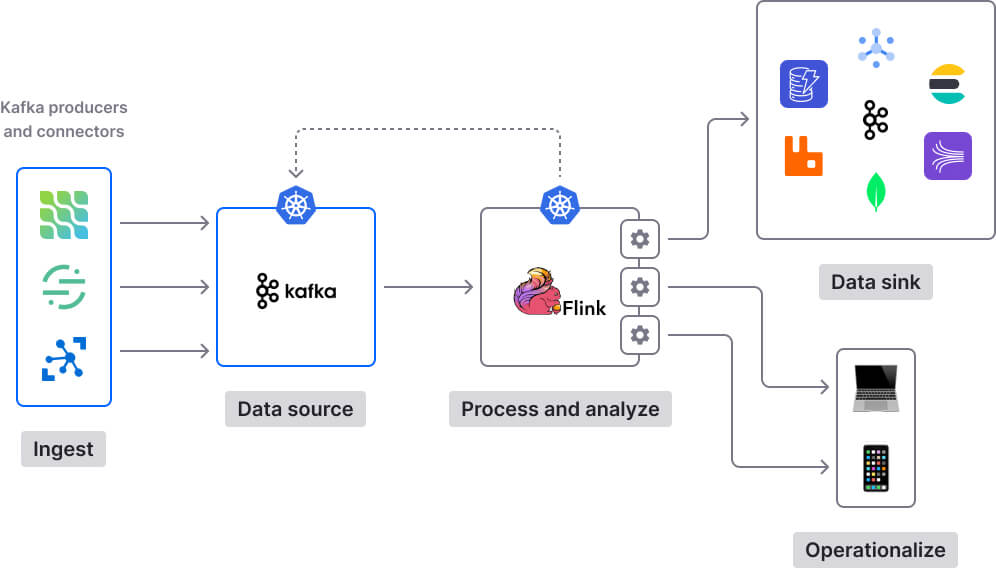
We’ll now look at what it takes to build a PyFlink pipeline that ingests data from a source, processes it, and then sends it to a destination. Flink natively supports various connectors for seamless integration with source and sink systems such as filesystems, Apache Kafka, Apache Cassandra, DynamoDB, Amazon Kinesis, RabbitMQ, and MongoDB. In addition to using pre-existing connectors, you can write your own custom ones. 

Learn more about:

• Table API connectors
• DataStream API connectors

We will go through a couple of basic examples, showing how to use PyFlink’s Table and DataStream APIs to read data from a Kafka topic, process it, and then send the output to another Kafka topic.

We’ll also review other aspects, such as logging and debugging your PyFlink programs, handling dependencies, and deploying PyFlink jobs to production. 

Note: If you’ve used Flink previously or if you have a good theoretical understanding of its features and capabilities, you will come across plenty of familiar concepts (since Flink is the underlying foundation for PyFlink). If you’re entirely new to Flink, it might be worth acquainting yourself with its basics (e.g., features, capabilities, architecture, key concepts) before diving into the PyFlink content below. 

Workflow, roles, and responsibilities

Before diving into hands-on examples and code, I think it’s worth discussing the workflow, roles, and responsibilities involved in bringing a PyFlink program from concept to production. 

The high-level PyFlink workflow generally looks like this:

1. Create a job (set up a sink and source, and implement your processing logic via PyFlink’s built-in capabilities or through custom UDFs). 
2. Run the job locally for testing purposes.
3. Debug, iterate, and optimize the job until you’re satisfied.
4. Deploy the job to a remote cluster for further testing and debugging.
5. Debug and optimize the job (again).
6. Deploy the job to production.
7. Manage the job in production (continuously monitor the job and debug it if necessary).

Getting a PyFlink pipeline from ideation to production involves a collaboration between different types of stakeholders. Ideally, all of the following roles are involved in creating and deploying PyFlink programs:

Exact responsibilities may differ from organization to organization. Large-scale enterprises may have all these roles, with clearly defined responsibilities.  However, in medium and early-stage companies, these roles and responsibilities are often conflated. For instance, in a start-up, a data engineer might also take on ML engineering tasks, while a software developer might additionally manage DevOps responsibilities like job deployment and infrastructure management. 

In any case, the takeaway is that working with PyFlink is not a one-person job. Quite the contrary. It’s a multi-step process that introduces operational complexity and requires cross-functional collaboration. You might even need a dedicated team (or teams!) to handle large-scale PyFLink deployments. 

Prerequisites

At the time of writing (March 2024), using PyFlink requires a Python version between 3.8 and 3.11. 

PyFlink is available on PyPi. Installing it is as simple as:

$ python -m pip install apache-flink

‍

You can also build your own custom PyFlink package for pip installation. To do so, follow these instructions. 

Creating a job using the PyFlink Table API

The PyFlink Table API uses a Domain-Specific Language (DSL) for defining table queries and transformations. While DSLs can offer benefits like higher abstraction levels and a more intuitive syntax for domain-specific tasks, they also have downsides:

• There’s a learning curve associated with any DSL.
• Integrating DSLs with other parts of a software system or with other tools and languages can be challenging.
• Users will likely encounter limitations when trying to implement functionality that goes beyond the scope of DSLs.

Before using the PyFflink Table API to implement a processing job, you must first create an execution environment (TableEnvironment). This is the main component within PyFlink's Table API for setting up, configuring, and executing table-based data transformations. Here’s a snippet demonstrating how to declare an execution environment:

env_settings = EnvironmentSettings.in_streaming_mode()
t_env = TableEnvironment.create(env_settings)

‍

After that’s done, you can create sink and source tables. As mentioned before, for our example, we will be consuming from and sending data to Kafka topics:

# Define the Kafka source table
t_env.create_temporary_table(
    'kafka_source',
    TableDescriptor.for_connector('kafka')
        .schema(Schema.new_builder()
                .column('transaction_id', DataTypes.STRING())
                .column('customer_id', DataTypes.STRING())
                .column('product_id', DataTypes.STRING())
                .column('quantity', DataTypes.INT())
                .column('price', DataTypes.FLOAT())
                .column('discount_code', DataTypes.STRING()) 
                .column('sales_rep_id', DataTypes.STRING())                   
                .build())
        .option('topic', 'transactions_topic')
        .option('properties.bootstrap.servers', 'localhost:9092')
        .option('properties.group.id', 'transaction_group')
        .option('scan.startup.mode', 'earliest-offset')
        .format(FormatDescriptor.for_format('json')
                .option('json.fail-on-missing-field', 'false')
                .option('json.ignore-parse-errors', 'true')
                .build())
        .build())

# Define the Kafka sink table
t_env.create_temporary_table(
    'kafka_sink',
    TableDescriptor.for_connector('kafka')
        .schema(Schema.new_builder()
                .column('transaction_id', DataTypes.STRING())
                .column('customer_id', DataTypes.STRING())
                .column('product_id', DataTypes.STRING())
                .column('quantity', DataTypes.INT())
                .column('price', DataTypes.FLOAT())
                .build())
        .option('topic', 'sales_report_topic')
        .option('properties.bootstrap.servers', 'localhost:9092')
        .format(FormatDescriptor.for_format('json')
                .build())
        .build())

‍

The code snippet above registers two tables, kafka_source and kafka_sink. The former consumes data from a Kafka topic named transactions_topic, while the latter writes data to another Kafka topic named sales_report_topic. 

After setting up the sink and source tables, you can implement your data processing logic. PyFlink’s Table API operators allow you to transform and manipulate tables. Numerous operators are available; for brevity, I won’t go through all of them here. Instead, I will list some of the main types of operations you can perform with them:

• Column operations (e.g., add, replace, remove, rename columns). 
• Row-based operations (e.g., map). 
• Aggregations such as grouping by clause and aggregating group rows.
• Joins (for example, inner, outer, and interval joins). 
• Windowing (e.g., sliding, tumbling, group windows). 

Refer to the documentation to see the entire list of operators available for the Table API, together with code snippets for each. 

Unlike operators, which are mainly used to shape the overall structure of your tables, functions generally allow you to transform the data in tables. PyFlink’s Table API offers numerous built-in functions. These enable a wide range of transformations, including string manipulations, mathematical calculations, date and time manipulation, type conversion, pattern matching, and the implementation of conditional logic.

You can even write custom UDFs to extend PyFlink’s Table API capabilities beyond built-in functions. These can be either standard UDFs, which process data one row at a time, or vectorized UDFs, which process data one batch at a time. A UDF can be further classified into one of the following categories:

• Scalar function. It maps zero, one, or multiple scalar values to a new scalar value. 
• Table function. It takes zero, one, or multiple scalar values as input and returns an arbitrary number of rows as output.  
• Aggregate function. It maps scalar values of multiple rows to a new scalar value. 
• Table aggregate function. It maps scalar values of multiple rows to zero, one, or multiple rows.

Anyway, going back to our example, let’s assume we want to drop a couple of columns (discount_code and sales_rep_id) from the kafka_source table (which reads from transactions_topic in Kafka). We can do that by using the drop_columns operator:

# Use the Table API to read from the source table
transactions = t_env.from_path("kafka_source")

# Drop the 'discount_code' and 'sales_rep_id' columns
sales_report = transactions.drop_columns(['discount_code', 'sales_rep_id'])

# Write the transformed data into the sink table
sales_report.execute_insert("kafka_sink").wait()

‍

The final line of code in the snippet above writes the result to the kafka_sink table. The use of execute_insert("kafka_sink") triggers the execution of the job, where the transformed data is inserted into the kafka_sink table (and from there, to the sales_report_topic in Kafka). 

To recap, here’s our end-to-end example:

import sys
from pyflink.table import EnvironmentSettings, TableEnvironment, DataTypes, Schema, FormatDescriptor, TableDescriptor

def retail_sales_report(input_topic, output_topic, bootstrap_servers):
    """
    A function to read transaction data from a Kafka topic, transform it by dropping specific columns, and write the transformed data to another Kafka topic for a retail sales report.
    """
    # Initialize the Table Environment
    env_settings = EnvironmentSettings.in_streaming_mode()
    t_env = TableEnvironment.create(env_settings)

    # Define the Kafka Source Table
    t_env.create_temporary_table(
        'kafka_source',
        TableDescriptor.for_connector('kafka')
            .schema(Schema.new_builder()
                    .column('transaction_id', DataTypes.STRING())
                    .column('customer_id', DataTypes.STRING())
                    .column('product_id', DataTypes.STRING())
                    .column('quantity', DataTypes.INT())
                    .column('price', DataTypes.FLOAT())
                    .column('discount_code', DataTypes.STRING()) 
                    .column('sales_rep_id', DataTypes.STRING())                   
                    .build())
            .option('topic', 'transactions_topic')
            .option('properties.bootstrap.servers', 'localhost:9092')
            .option('properties.group.id', 'transaction_group')
            .option('scan.startup.mode', 'earliest-offset')
            .format(FormatDescriptor.for_format('json')
                    .option('json.fail-on-missing-field', 'false')
                    .option('json.ignore-parse-errors', 'true')
                    .build())
            .build())

    # Define the Kafka Sink Table
    t_env.create_temporary_table(
        'kafka_sink',
        TableDescriptor.for_connector('kafka')
            .schema(Schema.new_builder()
                    .column('transaction_id', DataTypes.STRING())
                    .column('customer_id', DataTypes.STRING())
                    .column('product_id', DataTypes.STRING())
                    .column('quantity', DataTypes.INT())
                    .column('price', DataTypes.FLOAT())
                    .build())
            .option('topic', 'sales_report_topic')
            .option('properties.bootstrap.servers', 'localhost:9092')
            .format(FormatDescriptor.for_format('json')
                    .build())
            .build())

    # Read data from the Kafka source table
    transactions = t_env.from_path("kafka_source")

    # Apply transformation to drop 'discount_code' and 'sales_rep_id' columns
    sales_report = transactions.drop_columns(['discount_code', 'sales_rep_id'])

    # Write the transformed data into the Kafka sink table
    sales_report.execute_insert("kafka_sink").wait()

if __name__ == '__main__':
    if len(sys.argv) == 4:
        input_topic = sys.argv[1]
        output_topic = sys.argv[2]
        bootstrap_servers = sys.argv[3]
        retail_sales_report(input_topic, output_topic, bootstrap_servers)
    else:
        print("Usage: python retail_sales_report.py <input_topic> <output_topic> <bootstrap_servers>")

‍

You can execute jobs locally for testing and debugging purposes. For instance, if you name your job “sales_report_job.py”, this is how you do it:

$ python sales_report_job.py

‍

This will launch a local mini-cluster that runs in a single process to execute the PyFlink job. 

More information about deploying PyFlink jobs to remote clusters and production environments is available later in this article.  

Creating a job using the PyFlink DataStream API

The PyFlink DataStream API provides a lower-level abstraction for building real-time, event-driven applications. It enables detailed control over data streams and stateful computations. However, it has a steep learning curve; to make the most of it, users must understand concepts like checkpoints, savepoints and state management, which can be complex for newcomers. Learn more about:

• Stateful stream processing with (Py)Flink
• Building stateful programs with the DataStream API 

Additionally, deploying and managing stateful processing applications in production brings many challenges.  

Similar to the Table API, building a processing job with PyFlink’s DataStream API requires you to first declare an execution environment (StreamExecutionEnvironment):

env = StreamExecutionEnvironment.get_execution_environment()
env.set_parallelism(1)
env.set_runtime_mode(RuntimeExecutionMode.STREAMING)

‍

The StreamExecutionEnvironment is the central component responsible for creating, configuring, and executing streaming data applications, similar to the role played by the TableEnvironment in the Table API.

Once you have an execution environment, you can configure your source and sink. For our example, the source and sink point to Kafka topics:

# Define Kafka Source
source = KafkaSource.builder() \
    .set_bootstrap_servers("localhost:9092") \
    .set_topics("social_media_posts") \
    .set_group_id("analysis_group") \
    .set_starting_offsets(KafkaOffsetsInitializer.earliest()) \
    .set_value_only_deserializer(SimpleStringSchema()) \
    .build()

ds = env.from_source(source, WatermarkStrategy.for_monotonous_timestamps(), "Kafka Source")

# Define Kafka Sink
sink = KafkaSink.builder() \
    .set_bootstrap_servers("localhost:9092") \
    .set_record_serializer(
        KafkaRecordSerializationSchema.builder()
            .set_topic("sentiment_analysis_results")
            .set_value_serialization_schema(SimpleStringSchema())
            .build()
    ) \
    .set_delivery_guarantee(DeliveryGuarantee.AT_LEAST_ONCE) \
    .build()

stream.sink_to(sink)

‍

The code snippet above initializes a Kafka source to ingest data from a topic named social_media_posts and a Kafka sink to output data to a topic named sentiment_analysis_results.

Up next, let’s see what kind of processing we can do. PyFlink’s DataStream API operators enable us to implement transformations on data streams. Similar to the Table API, PyFlink’s DataStream API offers numerous operators. While I won't cover all of them, I'll highlight some key types of transformations you can perform:

• Map. Transform an element of the stream to another element.
• FlatMap. Similar to Map, but each input item can be transformed into zero, one, or more output items.
• Filter. Evaluate a boolean function for each element and retain those for which the function returns true.
• KeyBy. Logically partition the stream based on certain attributes; necessary for aggregations and keyed process functions.
• Reduce. Apply a reduce function to consecutive elements in a keyed stream to produce a rolling aggregation.
• Window Join. Join two streams on a key and a common window.
• Interval Join. Join two streams based on time boundaries.
• Windowing (tumbling, sliding, session, global windows). 

Check out this page to see the entire list of transformations available for the DataStream API, together with code examples for each.

It’s important to note that you can also use UDFs to customize and define the functionality of transformations to fit the specific needs and requirements of your application. There are several different ways to do so:

• Implement function interfaces (e.g., MapFunction is provided for the Map transformation, FilterFunction is provided for the Filter transformation, etc.).
• Define the functionality of the transformation through a Lambda function.
• Use a Python function to implement the logic of the transformation.

For our example, let’s assume we want to perform sentiment analysis on data coming from the Kafka source (the social_media_posts topic). To do so, we can use a UDF that customizes and implements the map transformation: 

class SentimentAnalysis(MapFunction):
    def map(self, value):
        # Example of simple sentiment analysis logic
        positive_keywords = ['happy', 'joyful', 'love']
        negative_keywords = ['sad', 'angry', 'hate']
        # Assuming 'value' is a text of the social media post
        post_text = value.lower()  # Convert to lowercase to simplify matching
        sentiment = "Neutral"  # Default sentiment
        for keyword in positive_keywords:
            if keyword in post_text:
                sentiment = "Positive"
                break  # Stop searching if any positive keyword is found
        for keyword in negative_keywords:
            if keyword in post_text:
                sentiment = "Negative"
                break  # Stop searching if any negative keyword is found
        return f"Post: {value} | Sentiment: {sentiment}"

processed_stream = ds.map(SentimentAnalysis(), output_type=Types.STRING())

‍

To submit the job for execution, you simply have to call env.execute().

Here’s what our end-to-end job looks like:

from pyflink.common.serialization import SimpleStringSchema
from pyflink.common.typeinfo import Types
from pyflink.datastream import StreamExecutionEnvironment
from pyflink.datastream.connectors import KafkaSource, KafkaSink, KafkaRecordSerializationSchema, DeliveryGuarantee
from pyflink.datastream.functions import MapFunction
from pyflink.common.watermark_strategy import WatermarkStrategy
from pyflink.datastream.connectors import KafkaOffsetsInitializer
from pyflink.datastream.execution_mode import RuntimeExecutionMode

def sentiment_analysis_job():
    """
    Sets up a PyFlink job that consumes social media posts from a Kafka   topic, performs sentiment analysis, and outputs results to another Kafka topic.
    """
    # Declare the execution environment.
    env = StreamExecutionEnvironment.get_execution_environment()
    env.set_parallelism(1)
    env.set_runtime_mode(RuntimeExecutionMode.STREAMING)

    # Define a source to read from Kafka.
    source = KafkaSource.builder() \
        .set_bootstrap_servers("localhost:9092") \
        .set_topics("social_media_posts") \
        .set_group_id("analysis_group") \
        .set_starting_offsets(KafkaOffsetsInitializer.earliest()) \
        .set_value_only_deserializer(SimpleStringSchema()) \
        .build()
    
    ds = env.from_source(source, WatermarkStrategy.for_monotonous_timestamps(), "Kafka Source")

    # Implement the custom SentimentAnalysis map function.
    class SentimentAnalysis(MapFunction):
        def map(self, value):
            # Keywords to determine post sentiment.
            positive_keywords = ['happy', 'joyful', 'love']
            negative_keywords = ['sad', 'angry', 'hate']
            # Default sentiment is Neutral.
            sentiment = "Neutral"
            post_text = value.lower()  # Compare in lowercase.
            for keyword in positive_keywords:
                if keyword in post_text:
                    sentiment = "Positive"
                    break
            for keyword in negative_keywords:
                if keyword in post_text:
                    sentiment = "Negative"
                    break
            return f"Post: {value} | Sentiment: {sentiment}"

    # Apply the map function to process each post.
    stream = ds.map(SentimentAnalysis(), output_type=Types.STRING())

    # Define a sink to write to Kafka.
    sink = KafkaSink.builder() \
        .set_bootstrap_servers("localhost:9092") \
        .set_record_serializer(
            KafkaRecordSerializationSchema.builder()
                .set_topic("sentiment_analysis_results")
                .set_value_serialization_schema(SimpleStringSchema())
                .build()
        ) \
        .set_delivery_guarantee(DeliveryGuarantee.AT_LEAST_ONCE) \
        .build()

    # Direct the processed data to the sink.
    stream.sink_to(sink)

    # Execute the job.
    env.execute()

if __name__ == "__main__":
    sentiment_analysis_job()

‍

The job will continuously consume social media posts from the source Kafka topic (social_media_posts) and perform sentiment analysis via the SentimentAnalysis class. SentimentAnalysis categorizes each post as "Positive," "Negative," or "Neutral" based on the presence of certain keywords. The output is a string that includes the original post text along with its determined sentiment. This output is sent to the sync Kafka topic (sentiment_analysis_results). This entire process happens in real time. 

But let’s take it one step further. Let’s say you not only want to classify each post, but you additionally want to apply 5-minute tumbling windows to count the number of posts per sentiment category within each window. This aggregation is useful for monitoring and analyzing evolving trends over time (and it’s a classical example of stateful stream processing). 

Here’s how we could adjust our existing job to incorporate these additions:

from pyflink.common.serialization import SimpleStringSchema
from pyflink.common.typeinfo import Types
from pyflink.datastream import StreamExecutionEnvironment, TimeCharacteristic
from pyflink.datastream.connectors import KafkaSource, KafkaSink, KafkaRecordSerializationSchema, DeliveryGuarantee
from pyflink.datastream.functions import MapFunction, ProcessWindowFunction, WindowFunction
from pyflink.datastream.window import TumblingProcessingTimeWindows
from pyflink.datastream.assigner import TumblingProcessingTimeWindows
from pyflink.common.time import Time
from pyflink.common.watermark_strategy import WatermarkStrategy
from pyflink.datastream.connectors import KafkaOffsetsInitializer
from pyflink.datastream.execution_mode import RuntimeExecutionMode
from pyflink.datastream.functions import ProcessAllWindowFunction, ProcessWindowFunction
from pyflink.datastream.window import TimeWindow
from pyflink.util.java_utils import JArrayList

def sentiment_analysis_job():
    """
    Sets up a PyFlink job that consumes social media posts from a Kafka topic, performs sentiment analysis, aggregates results in 5-minute windows, and sends the output to another Kafka topic.
    """
    # Declare the execution environment
    env = StreamExecutionEnvironment.get_execution_environment()
    env.set_parallelism(1)
    env.set_runtime_mode(RuntimeExecutionMode.STREAMING)

    # Define a source to read from Kafka
    source = KafkaSource.builder() \
        .set_bootstrap_servers("localhost:9092") \
        .set_topics("social_media_posts") \
        .set_group_id("analysis_group") \
        .set_starting_offsets(KafkaOffsetsInitializer.earliest()) \
        .set_value_only_deserializer(SimpleStringSchema()) \
        .build()

    ds = env.from_source(source, WatermarkStrategy.for_monotonous_timestamps(), "Kafka Source")

    # Implement the custom SentimentAnalysis map function
    class SentimentAnalysis(MapFunction):
        def map(self, value):
            # Keywords to determine post sentiment.
            positive_keywords = ['happy', 'joyful', 'love']
            negative_keywords = ['sad', 'angry', 'hate']
            # Default sentiment is Neutral.
            sentiment = "Neutral"
            post_text = value.lower()
            for keyword in positive_keywords:
                if keyword in post_text:
                    sentiment = "Positive"
                    break
            for keyword in negative_keywords:
                if keyword in post_text:
                    sentiment = "Negative"
                    break
            return f"Post: {value} | Sentiment: {sentiment}"

    # Apply the map function to process each post
    stream = ds.map(SentimentAnalysis(), output_type=Types.STRING())

    # Extract sentiment as key and apply windowing (NEW)
    def extract_sentiment(value):
        sentiment = value.split("|")[-1].strip().split(":")[-1].strip()
        return (sentiment, 1)

    keyed_stream = stream.map(extract_sentiment, output_type=Types.TUPLE([Types.STRING(), Types.INT()]))

    # Define a window function to count posts per sentiment (NEW)
    class CountSentiment(WindowFunction):
        def apply(self, key, window, input, out):
            count = sum([i[1] for i in input])
            out.collect((key, window.get_end(), count))

    # Apply tumbling window (NEW)
    windowed_stream = keyed_stream \
        .key_by(lambda x: x[0]) \
        .window(TumblingProcessingTimeWindows.of(Time.minutes(5))) \
        .apply(CountSentiment(), output_type=Types.TUPLE([Types.STRING(), Types.LONG(), Types.INT()]))

    # Define a sink to write to Kafka
    sink = KafkaSink.builder() \
        .set_bootstrap_servers("localhost:9092") \
        .set_record_serializer(
            KafkaRecordSerializationSchema.builder()
                .set_topic("sentiment_analysis_aggregations")
                .set_value_serialization_schema(SimpleStringSchema())
                .build()
        ) \
        .set_delivery_guarantee(DeliveryGuarantee.AT_LEAST_ONCE) \
        .build()

    # Direct the processed data to the sink
    windowed_stream.sink_to(sink)

    # Execute the job
    env.execute()

if __name__ == "__main__":
    sentiment_analysis_job()

‍

Once you’ve configured the job, you’re ready to test it. Similar to Table API jobs, you can execute DataStream API jobs locally for testing and debugging purposes: 

$ python sentiment_analysis_job.py

‍

This will launch a local mini-cluster that runs in a single process to execute the PyFlink job. 

Handling dependencies

Your PyFlink jobs may depend on external components (e.g., other Python libraries, ML frameworks, data storage solutions) that aren’t part of the Flink distribution. You must manage these dependencies to ensure your PyFlink job runs smoothly. 

PyFlink provides several ways to handle dependencies, which I will briefly present. 

Third-party JARs can be specified in the Table and DataStream APIs. Here’s an example showing how you can do that:

# Table API
table_env.get_config().set("pipeline.jars", "file:///my/jar/path/connector.jar;file:///my/jar/path/udf.jar")

# DataStream API
stream_execution_environment.add_jars("file:///my/jar/path/connector1.jar", "file:///my/jar/path/connector2.jar")

‍

Similar to JARs, Python libraries can also be configured via the Table and DataStream APIs as dependencies:

# Table API
table_env.add_python_file(file_path)


# DataStream API
stream_execution_environment.add_python_file(file_path)

‍

Alternatively, third-party Python dependencies can be specified via a requirements.txt file.  

Note that using Python libraries within PyFlink involves writing UDFs that allow you to extend the capabilities of PyFlink by incorporating custom logic. This is a powerful feature, as it opens up the vast ecosystem of Python libraries for tasks such as data manipulation, machine learning, and statistical analysis directly within your PyFlink data pipelines. However, this also brings some challenges:

• Invoking Python UDFs adds a performance overhead that can affect the latency and throughput of your data processing tasks, especially for high-volume or low-latency requirements.
• Debugging and testing UDFs is more complex than using Flink’s built-in operators and functions. 
• Writing UDFs can be a time-consuming, laborious task. 

Going beyond Python libraries, PyFlink allows you to specify archive files and Python interpreters (for executing Python workers and parsing Python UDFs on the client side) as dependencies in your code. Read the PyFlink Dependency Management documentation page to find out more.

Note: If you are using both the DataStream API and the Table API in a single job, it’s enough to specify the dependencies via the DataStream API to ensure they work for both APIs.  

All the dependencies I’ve presented above can also be passed through command line arguments in the Flink CLI when submitting the job. 

Data conversions

PyFlink supports several types of conversions. First of all, you can convert Pandas DataFrames to PyFlink tables and the other way around. This offers a way to port data and leverage the strengths of both tools — Pandas for complex data manipulation and analysis tasks and PyFlink for scalable data processing. However, bear in mind that converting between Pandas DataFrames and PyFlink tables can introduce a performance overhead (due to serialization and deserialization of data). Additionally, you might encounter data compatibility issues, and you’ll have a more complex workflow. 

The following example shows how to create a PyFlink table from a Pandas DataFrame:

from pyflink.table import DataTypes

import pandas as pd
import numpy as np

# Create a Pandas DataFrame
pdf = pd.DataFrame(np.random.rand(1000, 2))

# Create a PyFlink Table from a Pandas DataFrame
table = t_env.from_pandas(pdf)

# Create a PyFlink Table from a Pandas DataFrame with the specified column names
table = t_env.from_pandas(pdf, ['f0', 'f1'])

# Create a PyFlink Table from a Pandas DataFrame with the specified column types
table = t_env.from_pandas(pdf, [DataTypes.DOUBLE(), DataTypes.DOUBLE()])

# Create a PyFlink Table from a Pandas DataFrame with the specified row type
table = t_env.from_pandas(pdf,
                          DataTypes.ROW([DataTypes.FIELD("f0", DataTypes.DOUBLE()),
                                         DataTypes.FIELD("f1", DataTypes.DOUBLE())]))

‍

And this is how you convert a PyFlink table to a Pandas DataFrame:

from pyflink.table.expressions import col

import pandas as pd
import numpy as np

# Create a PyFlink Table
pdf = pd.DataFrame(np.random.rand(1000, 2))
table = t_env.from_pandas(pdf, ["a", "b"]).filter(col('a') > 0.5)

# Convert the PyFlink Table to a Pandas DataFrame
pdf = table.limit(100).to_pandas()

‍

Secondly, PyFlink allows you to convert a table into a DataStream and vice versa. This is useful for scenarios where you might use the Table API alongside the DataStream API as part of your data processing pipeline. For example, you could rely on the Table API for some initial stateless data normalization and cleansing before implementing the main stateful data processing pipeline with the DataStream API. Similar to porting data between PyFlink tables and Pandas DataFrames, the ability to convert between tables and DataStreams can impact performance and lead to increased complexity. 

Debugging PyFlink jobs

To help with debugging, PyFlink applications support both client-side and server-side logging. You can use print statements and standard Python logging modules to log contextual and debug information (outside of UDF code). 

Here’s an example of how to add logging to the client side:

import logging
logging.warning(table.get_schema())

# use print function
print(table.get_schema())

‍

Client logs will appear in the client's log files during job submission.

And here’s a snippet demonstrating how to implement logging on the server side:

import logging

@udf(result_type=DataTypes.BIGINT())
def add(i, j):
    # use logging modules
    logging.info("debug")
    # use print function
    print('debug')
    return i + j

‍

These server logs will appear in the log files of the TaskManagers during job execution. 

If the FLINK_HOME environment variable is set, logs will be written in the log directory under FLINK_HOME. Otherwise, logs will be written to the PyFlink module directory.   

You can debug Python UDFs either locally or remotely: 

• Local debugging implies debugging your functions directly in an IDE (such as PyCharm, PyDev, Wing Python IDE, or VS Code, to name just a few).
• Remote debugging can be done by using the pydevd_pycharm debugger. See these instructions for details. 

In some scenarios, Java knowledge might be required in addition to Python to perform debugging. That’s because Flink is fundamentally a Java technology, while PyFlink is just a wrapper around it. For example, if your PyFlink application experiences performance slowdowns or memory leaks, the issue might stem from the way Python processes interact with Java processes. Debugging the Java side could help you understand how resources are being managed and how data is being passed between the Python and Java layers, potentially uncovering inefficiencies or bugs in the JVM or the Flink Java codebase. 

In practice, if you’re a data scientist, developer, or ML engineer who knows Python but not Java, you may need to collaborate with Java developers to debug your PyFlink programs.

Deploying PyFlink jobs to remote and production-ready clusters

After you’ve configured and tested your PyFlink job locally, it’s time to move it to a remote environment for further testing and, eventually, production.  

You can submit PyFlink jobs to remote clusters (standalone, YARN, or Kubernetes) for execution via the Flink CLI. Here’s an example demonstrating how to run a job on a remote Kubernetes cluster:

$ ./bin/flink run-application \
      --target kubernetes-application \
      --parallelism 8 \
      -Dkubernetes.cluster-id=<ClusterId> \
      -Dtaskmanager.memory.process.size=4096m \
      -Dkubernetes.taskmanager.cpu=2 \
      -Dtaskmanager.numberOfTaskSlots=4 \
      -Dkubernetes.container.image.ref=<PyFlinkImageName> \
      --pyModule sales_report_job \
      --pyFiles /opt/flink/usrlib/sales_report_job.py

‍

More examples are available here.

When working with UDFs, there are two different runtime execution modes to choose from:

• process. UDFs are executed in separate Python processes. This mode offers better resource isolation. 
• thread. UDFs are executed in threads within the Flink JVM process. This option ensures higher throughput and lower latencies. 

The following snippet shows how to specify what execution mode you want to use:

## Python Table API
# Specify `PROCESS` mode
table_env.get_config().set("python.execution-mode", "process")
# Specify `THREAD` mode
table_env.get_config().set("python.execution-mode", "thread")

## Python DataStream API
config = Configuration()
# Specify `PROCESS` mode
config.set_string("python.execution-mode", "process")
# Specify `THREAD` mode
config.set_string("python.execution-mode", "thread")
# Create the corresponding StreamExecutionEnvironment
env = StreamExecutionEnvironment.get_execution_environment(config)

Scalability, fault tolerance, and monitoring in PyFlink

PyFlink leverages Flink’s scalability and fault tolerance capabilities. It supports elastic scaling, which allows the system to dynamically adjust computational resources in response to workload changes. PyFlink can scale to process up to petabytes of data per day, across hundreds or even thousands of nodes. 

For fault tolerance, PyFlink employs checkpoints and savepoints. Checkpoints periodically and automatically capture the state of processing tasks. This allows for recovery from failures by restoring to the most recent checkpoint. Meanwhile, savepoints are triggered manually to create snapshots of the application's state. They’re mostly used for planned operations (e.g., updating the Flink version). 

PyFlink also inherits Flink’s monitoring capabilities. Internally, Flink provides metrics accessible via its web UI, including job throughput, latency, operator backpressure, and memory usage, which are essential for identifying bottlenecks and optimizing PyFlink applications. Additionally, (Py)Flink’s metrics system can be extended to external monitoring tools such as Prometheus and Grafana.

Ensuring robust monitoring, effective scaling, and fault tolerance for PyFlink applications in production are some of the greatest operational challenges of working with PyFlink. Dealing with these challenges requires a significant time investment and ongoing financial costs. 

PyFlink’s architecture and internals

Let’s now take a look at how PyFlink works under the hood. Specifically, at how jobs are compiled and then executed. First, though, I suggest you familiarize yourself with Flink’s architecture (in case you aren’t already). It’s important to understand Flink’s internals before delving into PyFlink, as PyFlink builds upon them. 

The key thing to bear in mind is that PyFlink is not a rewrite of the Flink engine in Python. Instead, it’s a wrapper around Flink’s Java computing engine. 

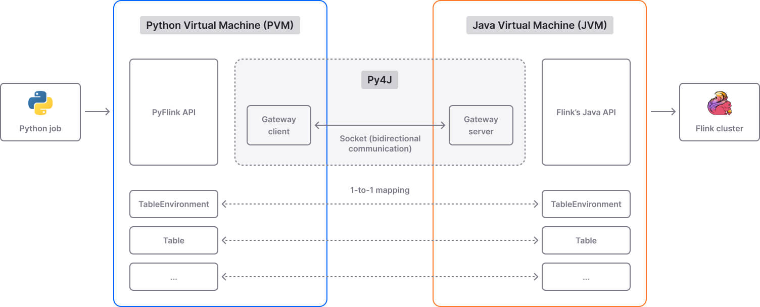
Job compiling

PyFlink reuses the existing job compiling stack of Flink’s Java API. PyFlink and the Flink Java API expose equivalent classes and objects (e.g., TableEnvironment). When a Python program makes a PyFlink API call, a corresponding Java object is created in the JVM and the method is called on it. Communication between the Python Virtual Machine (PVM) and Java Virtual Machine (JVM) layers is powered by Py4J. 

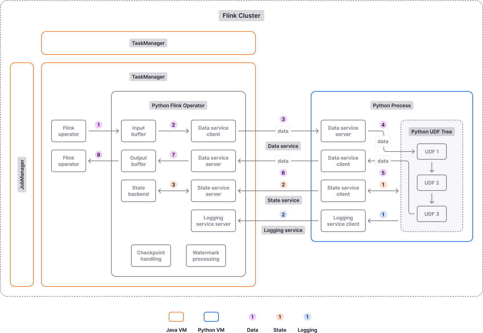
Job execution

A Flink job is typically composed of a sequence of data transformations, where each transformation is represented by an operator. Once you submit the job to a Flink cluster, JobManager assigns the job’s operators to TaskManager for execution. 

As I mentioned earlier in this article, when working with Python UDFs, there are two execution modes to choose from: process and thread. 

In process mode, special Python operators are used to handle Python UDFs. This is needed because Python UDFs are executed by processes running on Python workers. The communication between JVM and PVM is achieved through various gRPC services (e.g., DataService manages the transfer of business data) that are built using Apache Beam's Fn APIs.  

Executing Python UDFs in separate Python processes adds serialization/deserialization and communication overhead, leading to extra latency. That’s why starting with Apache Flink version 1.15, the thread execution mode was introduced. This new mode allows Python UDFs to be executed in the JVM as a thread instead of a separate Python process, which leads to lower latency and better throughput. However, it has its drawbacks too. For example, it only supports the CPython interpreter, and it offers reduced isolation compared to the process mode. To learn more about thread and process mode and when it’s best to use each, check out this article. 

PyFlink: the good and the bad 

I’ve already mentioned (or implied) some of PyFlink’s advantages and disadvantages throughout this article, but I think it’s worth collating them here to refresh our memories. They are key aspects you will have to consider if you are pondering whether or not to adopt PyFlink.   

Let’s start with the pros of using (Py)Flink:

• Makes Flink’s features accessible to Python users (developers, engineers and to a lesser extent, data scientists).  
• Versatile data processing framework, suitable for streaming, batch and, hybrid workloads.
• Rich stream processing capabilities, such as complex event-time processing, windowing, and state management. 
• Supports Python UDFs, which allows you to implement custom processing logic. 
• Scalable (up to thousands of nodes running in parallel) and able to handle large volumes of high-velocity data with low latency (in the millisecond range). 
• Can be used in conjunction with Python libraries like Pandas and NumPy.
• Integrates with a variety of tools and systems through sink and source connectors, including streaming platforms like Apache Kafka, message queues (e.g., RabbitMQ), and databases (for instance, MongoDB).

And here are the cons of using PyFlink:

• The PyFlink Table API is effectively a query language that executes standard operations by compiling them to Java at runtime. This is very limiting to Python developers who won’t be free to use their own classes, methods, or external libraries. 
• The PyFlink DataStream API allows you to execute dependencies such as third-party Python libraries and ML models, however the documentation is limited and it’s very difficult to understand how to make use of the capability. Basically, you can create a UDF to execute your ML model in a SQL-style query, but it’s not intuitive.
• PyFlink is essentially a wrapper around Flink’s Java APIs. While it’s great that you can write your code in Python, you will sometimes need Java expertise for debugging. It would be much more convenient and efficient if you could code and debug in the same language.
• PyFlink bridges Python's runtime with the Java Virtual Machine (JVM) where Flink operates. This requires data serialization and deserialization between Python and Java, leading to additional computational costs and potential bottlenecks, especially in high-throughput scenarios.
• When new Flink features or improvements are launched, these updates are generally first available in the Java API, and only later added to the Python API. So it’s safe to expect a feature parity gap between Flink’s Java API and PyFlink. 
• The learning curve for PyFlink can be steep. Depending on the team's prior experience with stream processing and distributed systems, this can take anywhere from a few weeks to a few months. 
• Setting up and configuring a (Py)Flink pipeline can be difficult, time-consuming, and expensive, often requiring a dedicated team. For instance, the Contentsquare engineering team worked for a year (!) to migrate from Spark to Flink and ensure everything worked as intended; it was a road riddled with challenges and gotchas they wished they had known earlier. 
• Considering its steep learning curve and complexity, it’s probably not cost-efficient to use (Py)Flink for small and medium workloads. 

PyFlink alternatives

Due to Flink’s proven capabilities and growing popularity, PyFlink is certainly worth considering if you are specifically interested in big data processing with Python. But other similar solutions are worth investigating too. Noteworthy Python alternatives to PyFlink include Apache Spark (PySpark), Faust, and Bytewax. I encourage you to assess them all before deciding which technology best suits your needs.

Another alternative to PyFlink is Quix Streams, an open-source library for building containerized stream processing applications with Python and Apache Kafka. In a nutshell, Quix Streams brings the following benefits:

• No JVM, no orchestrator, no server-side engine.
• Easily integrates with the entire Python ecosystem (pandas, scikit-learn, TensorFlow, PyTorch, etc).
• Support for many serialization formats, including JSON (and Quix-specific).
• Support for stateful operations using RocksDB.
• A simple framework with a Pandas-like interface to ease newcomers to streaming.
• "At-least-once" Kafka processing guarantees.
• Designed to run and scale resiliently via container orchestration (e.g., Kubernetes).
• Easily runs locally and in Jupyter Notebook for convenient development and debugging.

In addition, Quix Streams seamlessly integrates with Quix Cloud, which provides fully managed containers, Kafka, and observability tools. By pairing Quix Streams with Quix Cloud, you can build, deploy, and monitor Python stream processing apps without the headache of managing the underlying infrastructure. To learn more about Quix and what it can do for you, check out:

• The gallery of Quix sample projects. These are fully functioning event-driven applications that you can use to figure out what is possible with Quix, how Quix works, and how to start building your own projects.‍